ModelicaReference.Operators

In this chapter operators of Modelica are documented. Elementary operators, such as "+" or "-" are overloaded and operate on scalar and array variables. Other operators have the same syntax as a Modelica function call. However, they do not behave as a Modelica function, either because the result depends not only on the input arguments but also on the status of the simulation (such as "pre(..)"), or the function operates on input arguments of different types (such as "String(..)"). Neither of these "functions" can be defined with a "standard" Modelica function and are therefore builtin operators of the Modelica language (with exception of the basic mathematical functions, sin, cos, tan, asin, acos, atan, atan2, sinh, cosh, tanh, exp, log, log10 that are provided for convenience as built-in functions).

Extends from ModelicaReference.Icons.Information (Icon for general information packages).

Package Content

Name	Description
ElementaryOperators	Elementary operators (+, >, or, ..)
'abs()'	abs()
'acos()'	acos()
'actualStream()'	actualStream()
'array()'	array()
'asin()'	asin()
'assert()'	assert()
'atan()'	atan()
'atan2()'	atan2()
'cardinality()'	cardinality()
'cat()'	cat()
'ceil()'	ceil()
'change()'	change()
'connect()'	connect()
'Connections.branch()'	Connections.branch()
'Connections.root()'	Connections.root()
'Connections.potentialRoot()'	Connection.potentialRoot()
'Connections.isRoot()'	Connections.isRoot()
'Connections.rooted()'	Connections.rooted()
'cos()'	cos()
'cosh()'	cosh()
'cross()'	cross()
'delay()'	delay()
'der()'	der()
'diagonal()'	diagonal()
'div()'	div()
'edge()'	edge()
'exp()'	exp()
'fill()'	fill()
'floor()'	floor()
'homotopy()'	homotopy()
'identity()'	identity()
'initial()'	initial()
'inStream()'	inStream()
'Integer()'	Integer()
'integer()'	integer()
'linspace()'	linspace()
'log()'	log()
'log10()'	log10()
'matrix()'	matrix()
'max()'	max()
'min()'	min()
'mod()'	mod()
'ndims()'	ndims()
'noEvent()'	noEvent()
'ones()'	ones()
'outerProduct()'	outerProduct()
'pre()'	pre()
'product()'	product()
'reinit()'	reinit()
'rem()'	rem()
'rooted()'	rooted() - deprecated
'sample()'	sample()
'scalar()'	scalar()
'semiLinear()'	semiLinear()
'sign()'	sign()
'sin()'	sin()
'sinh()'	sinh()
'size()'	size()
'skew()'	skew()
'smooth()'	smooth()
'sqrt()'	sqrt()
'String()'	String()
'sum()'	sum()
'symmetric()'	symmetric()
'tan()'	tan()
'tanh()'	tanh()
'terminal()'	terminal()
'terminate()'	terminate()
'transpose()'	transpose()
'vector()'	vector()
'zeros()'	zeros()

ModelicaReference.Operators.ElementaryOperators

Elementary operators are overloaded and operate on variables of type Real, Integer, Boolean, and String, as well as on scalars or arrays.

Syntax

Arithmetic Operators (operate on Real, Integer scalars or arrays)
Operators	Example	Description
+, -, .+, .-	a + b a .+ b	addition and subtraction; element-wise on arrays
*	a * b	multiplication; scalararray: element-wise multiplication vectorvector: element-wise multiplication (result: scalar) matrixmatrix: matrix product vectormatrix: row-matrixmatrix (result: vector) matrixvector: matrix*column-matrix (result: vector)
/	a / b	division of two scalars or an array by a scalar; division of an array by a scalar is defined element-wise. The result is always of real type. In order to get integer division with truncation use the function div.
^	a^b	scalar power or integer power of a square matrix
.*, ./, .^	a .* b	element-wise multiplication, division and exponentiation of scalars and arrays
=	a * b = c + d	equal operator of an equation; element-wise on arrays
:=	a := c + d	assignment operator; element-wise on arrays

Relational Operators (operate on Real, Integer, Boolean, String scalars)
Operators	Example	Description
==	a == b	equal; for strings: identical characters
<>	a <> b	not equal; for strings: a is lexicographically less than b
<	a < b	less than
<=	a <= b	less than or equal
>	a > b	greater than
>=	a >= b	greater than or equal

Boolean Operators (operate on scalars or element-wise on arrays)
Operators	Example	Description
and	a and b	logical and
or	a or b	logical or
not	not a	logical not

Other Operators
Operators	Example	Description
[..]	[1,2;3,4]	Matrix constructor; "," separates columns, ";" separates rows
{..}	{{1,2}, {3,4}}	Array constructor; every {..} adds one dimension
"..."	"string value" "string "value""	String literal (" is used inside a string for ")
+	"abc" + "def"	Concatenation of string scalars or arrays

Operator precedence determines the order of evaluation of operators in an expression. An operator with higher precedence is evaluated before an operator with lower precedence in the same expression.

The following table presents all the expression operators in order of precedence from highest to lowest. All operators are binary except exponentiation, the postfix operators and those shown as unary together with expr, the conditional operator, the array construction operator {} and concatenation operator [ ], and the array range constructor which is either binary or ternary. Operators with the same precedence occur at the same line of the table:

Operator Group	Operator Syntax	Examples
postfix array index operator	`[]`	`arr[index]`
postfix access operator	`.`	`a.b`
postfix function call	funcName(function-arguments)	`sin(4.36)`
array construct/concat	{expressions} [expressions] [expressions; expressions...]	`{2,3} [5,6] [2,3; 7,8]`
exponentiation	`^`	`2^3`
multiplicative and array elementwise multiplicative	`* / .* ./`	`23 2/3 [1,2;3,4].[2,3;5,6]`
additive and array elementwise additive	`+ - +expr -expr .+ .-`	`a+b, a-b, +a, -a [1,2;3,4].+[2,3;5,6]`
relational	`< <= > >= == <>`	`a<b, a<=b, a>b, ...`
`...`
unary negation	`not expr`	`not b1`
logical and	`and`	`b1 and b2`
logical or<	`or`	`b1 or b2`
array range	expr `:` expr `:` expr	`1:5:100`, start:step:stop
conditional	`if` expr `then` expr `else` expr	`if b then 3 else x`
named argument	ident `=` expr	`x = 2.26`

The conditional operator may also include elseif-clauses. Equality = and assignment := are not expression operators since they are allowed only in equations and in assignment statements respectively. All binary expression operators are left associative.

Note, the unary minus and plus in Modelica is slightly different than in Mathematica (Mathematica is a registered trademark of Wolfram Research Inc.) and in MATLAB (MATLAB is a registered trademark of MathWorks Inc.), since the following expressions are illegal (whereas in Mathematica and in MATLAB these are valid expressions):

  2*-2   // = -4 in Mathematica/MATLAB; is illegal in Modelica
  --2    // =  2 in Mathematica/MATLAB; is illegal in Modelica
  ++2    // =  2 in Mathematica/MATLAB; is illegal in Modelica
  2--2   // =  4 in Mathematica/MATLAB; is illegal in Modelica

Extends from ModelicaReference.Icons.Information (Icon for general information packages).

ModelicaReference.Operators.'abs()'

Absolute value of Real or Integer variable.

Syntax

abs(v)

Description

Is expanded into "noEvent(if v ≥ 0 then v else -v)". Argument v needs to be an Integer or Real expression.

Examples

  abs({-3, 0, 3})
 = {3, 0, 3}

Extends from ModelicaReference.Icons.Information (Icon for general information packages).

ModelicaReference.Operators.'acos()'

Trigonometric inverse cosine function

Syntax

acos(u)

Description

Returns the inverse of cos of u, with -1 ≤ u ≤ +1. Argument u needs to be an Integer or Real expression.

The acos function can also be accessed as Modelica.Math.acos.

Examples

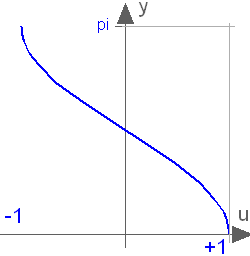
acos(0)
 = 1.5707963267949

Extends from ModelicaReference.Icons.Information (Icon for general information packages).

ModelicaReference.Operators.'actualStream()'

The actualStream(v) operator is provided for convenience, in order to return the actual value of the stream variable, depending on the actual flow direction. The only argument of this built-in operator needs to be a reference to a stream variable. The operator is vectorizable, in the case of vector arguments. For the following definition it is assumed that an (inside or outside) connector c contains a stream variable h_outflow which is associated with a flow variable m_flow in the same connector c:

actualStream(port.h_outflow) = if port.m_flow > 0 then inStream(port.h_outflow)
                                                  else port.h_outflow;

Example

The actualStream(v) operator is typically used in two contexts:

der(U) = c.m_flow*actualStream(c.h_outflow); // (1)energy balance equation
h_port = actualStream(port.h);               // (2)monitoring the enthalpy at a port

In the case of equation (1), although the actualStream() operator is discontinuous, the product with the flow variable is not, because actualStream()) is discontinuous when the flow is zero by construction. Therefore, a tool might infer that the expression is smooth(0, ...) automatically, and decide whether or not to generate an event. If a user wants to avoid events entirely, he/she may enclose the right-hand side of (1) with the noEvent() operator.

Equations like (2) might be used for monitoring purposes (e.g. plots), in order to inspect what the actual enthalpy of the fluid flowing through a port is. In this case, the user will probably want to see the change due to flow reversal at the exact instant, so an event should be generated. If the user does not bother, then he/she should enclose the right-hand side of (2) with noEvent(). Since the output of actualStream() will be discontinuous, it should not be used by itself to model physical behaviour (e.g., to compute densities used in momentum balances) - inStream() should be used for this purpose. The operator actualStream() should be used to model physical behaviour only when multiplied by the corresponding flow variable (like in the above energy balance equation), because this removes the discontinuity.

Extends from ModelicaReference.Icons.Information (Icon for general information packages).

ModelicaReference.Operators.'array()'

The constructor function array(A,B,C,...) constructs an array from its arguments.

Examples

{1,2,3} is a 3-vector of type Integer
{{11,12,13}, {21,22,23}} is a 2x3 matrix of type Integer
{{{1.0, 2.0, 3.0}}} is a 1x1x3 array of type Real

Real[3] v = array(1, 2, 3.0);
type Angle = Real(unit="rad");
parameter Angle alpha = 2.0; // type of alpha is Real.
// array(alpha, 2, 3.0) or {alpha, 2, 3.0} is a 3-vector of type Real.
Angle[3] a = {1.0, alpha, 4}; // type of a is Real[3].

Description

The constructor function array(A,B,C,...) constructs an array from its arguments according to the following rules:

Size matching: All arguments must have the same sizes, i.e., size(A)=size(B)=size(C)=...
All arguments must be type compatible expressions giving the type of the elements. The data type of the result array is the maximally expanded type of the arguments. Real and Integer subtypes can be mixed resulting in a Real result array where the Integer numbers have been transformed to Real numbers.
Each application of this constructor function adds a one-sized dimension to the left in the result compared to the dimensions of the argument arrays, i.e., ndims(array(A,B,C)) = ndims(A) + 1 = ndims(B) + 1, ...
{A, B, C, ...} is a shorthand notation for array(A, B, C, ...).
There must be at least one argument [i.e., array() or {} are not defined].

Extends from ModelicaReference.Icons.Information (Icon for general information packages).

ModelicaReference.Operators.'asin()'

Trigonometric inverse sine function

Syntax

asin(u)

Description

Returns the inverse of sin of u, with -1 ≤ u ≤ +1. Argument u needs to be an Integer or Real expression.

The asin function can also be accessed as Modelica.Math.asin.

Examples

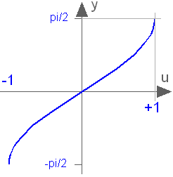
asin(0)
 = 0.0

Extends from ModelicaReference.Icons.Information (Icon for general information packages).

ModelicaReference.Operators.'assert()'

Trigger error and print error message if assertion condition is not fulfilled

Syntax

assert(condition, message, level = AssertionLevel.error)

Description

The Boolean expression condition shall be true for successful model evaluations. Otherwise, an error occurs using the string expression message as error message.

If the condition of an assert statement is true, message is not evaluated and the procedure call is ignored. If the condition evaluates to false different actions are taken depending on the level input:

level = AssertionLevel.error:
The current evaluation is aborted. The simulation may continue with another evaluation [e.g., with a shorter step-size, or by changing the values of iteration variables]. If the simulation is aborted, message indicates the cause of the error. Failed assertions takes precedence over successful termination, such that if the model first triggers the end of successful analysis by reaching the stop-time or explicitly with terminate(), but the evaluation with terminal()=true triggers an assert, the analysis failed.
level = AssertionLevel.warning:
The current evaluation is not aborted, message indicates the cause of the warning [It is recommended to report the warning only once when the condition becomes false, and it is reported that the condition is no longer violated when the condition returns to true. The assert(..) statement shall have no influence on the behavior of the model. For example, by evaluating the condition and reporting the message only after accepted integrator steps. The condition needs to be implicitly treated with noEvent(..) since otherwise events might be triggered that can lead to slightly changed simulation results].

The AssertionLevel.error case can be used to avoid evaluating a model outside its limits of validity; for instance, a function to compute the saturated liquid temperature cannot be called with a pressure lower than the triple point value. The AssertionLevel.warning case can be used when the boundary of validity is not hard: for instance, a fluid property model based on a polynomial interpolation curve might give accurate results between temperatures of 250 K and 400 K, but still give reasonable results in the range 200 K and 500 K. When the temperature gets out of the smaller interval, but still stays in the largest one, the user should be warned, but the simulation should continue without any further action. The corresponding code would be

  assert(T > 250 and T < 400, "Medium model outside full accuracy range",
         AssertionLevel.warning);
  assert(T > 200 and T < 500, "Medium model outside feasible region");

Examples

  parameter Real upperLimit=2;
  parameter Real lowerLimit=-2;
equation
  assert(upperLimit > lowerLimit, "upperLimit must be greater than lowerLimit.");

Extends from ModelicaReference.Icons.Information (Icon for general information packages).

ModelicaReference.Operators.'atan()'

Trigonometric inverse tangent function

Syntax

atan(u)

Description

Returns the inverse of tan of u, with -∞ < u < ∞. Argument u needs to be an Integer or Real expression.

The atan function can also be accessed as Modelica.Math.atan.

Examples

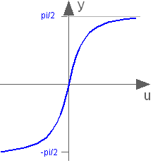
atan(1)
 = 0.785398163397448

Extends from ModelicaReference.Icons.Information (Icon for general information packages).

ModelicaReference.Operators.'atan2()'

Four quadrant inverse tangent

Syntax

atan2(u1,u2)

Description

Returns y = atan2(u1,u2) such that tan(y) = u1/u2 and y is in the range -pi < y ≤ pi. u2 may be zero, provided u1 is not zero. Usually u1, u2 is provided in such a form that u1 = sin(y) and u2 = cos(y). Arguments u1 and u2 need to be Integer or Real expressions.

The atan2 function can also be accessed as Modelica.Math.atan2.

Examples

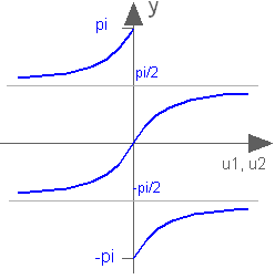
atan2(1,0)
 = 1.5707963267949

Extends from ModelicaReference.Icons.Information (Icon for general information packages).

ModelicaReference.Operators.'cardinality()'

Number of connectors in connection. This is a deprecated operator. It should no longer be used, since it will be removed in one of the next Modelica releases.

Syntax

cardinality(c)

Description

Returns the number of (inside and outside) occurrences of connector instance c in a connect statement as an Integer number.

[The cardinality operator allows the definition of connection dependent equations in a model.]

Instead of the cardinality(..) operator, often conditional connectors can be used, that are enabled/disabled via Boolean parameters.

Examples

connector Pin
  Real      v;
  flow Real i;
end Pin;
model Resistor
   Pin p, n;
equation
   // Handle cases if pins are not connected
      if cardinality(p) == 0 and cardinality(n) == 0 then
         p.v = 0;
         n.v = 0;
      elseif cardinality(p) == 0 then
         p.i = 0;
      elseif cardinality(n) == 0 then
         n.i = 0;
      end if;
   // Equations of resistor
      ...
end Resistor;

Extends from ModelicaReference.Icons.Information (Icon for general information packages).

ModelicaReference.Operators.'cat()'

The function cat(k,A,B,C,...)concatenates arrays A,B,C,... along dimension k.

Examples

Real[2,3] r1 = cat(1, {{1.0, 2.0, 3}}, {{4, 5, 6}});
Real[2,6] r2 = cat(2, r1, 2*r1);

Description

The function cat(k,A,B,C,...)concatenates arrays A,B,C,... along dimension k according to the following rules:

Arrays A, B, C, ... must have the same number of dimensions, i.e., ndims(A) = ndims(B) = ...
Arrays A, B, C, ... must be type compatible expressions giving the type of the elements of the result. The maximally expanded types should be equivalent. Real and Integer subtypes can be mixed resulting in a Real result array where the Integer numbers have been transformed to Real numbers.
k has to characterize an existing dimension, i.e., 1 <= k <= ndims(A) = ndims(B) = ndims(C); k shall be an integer number.
Size matching: Arrays A, B, C, ... must have identical array sizes with the exception of the size of dimension k, i.e., size(A,j) = size(B,j), for 1 <= j <= ndims(A) and j <> k.

Concatenation is formally defined according to:

Let R = cat(k,A,B,C,...), and let n = ndims(A) = ndims(B) = ndims(C) = ...., then
size(R,k) = size(A,k) + size(B,k) + size(C,k) + ...
size(R,j) = size(A,j) = size(B,j) = size(C,j) = ...., for 1 <= j <= n and j <> k.
R[i_1, ..., i_k, ..., i_n] = A[i_1, ..., i_k, ..., i_n], for i_k <= size(A,k),
R[i_1, ..., i_k, ..., i_n] = B[i_1, ..., i_k - size(A,i), ..., i_n], for i_k <= size(A,k) + size(B,k),
....
where 1 <= i_j <= size(R,j) for 1 <= j <= n.

Extends from ModelicaReference.Icons.Information (Icon for general information packages).

ModelicaReference.Operators.'ceil()'

Round a Real number towards plus infinity

Syntax

ceil(x)

Description

Returns the smallest integer not less than x. Result and argument shall have type Real. [Note, outside of a when clause state events are triggered when the return value changes discontinuously.]

Examples

ceil({-3.14, 3.14})
 = {-3.0, 4.0}

Extends from ModelicaReference.Icons.Information (Icon for general information packages).

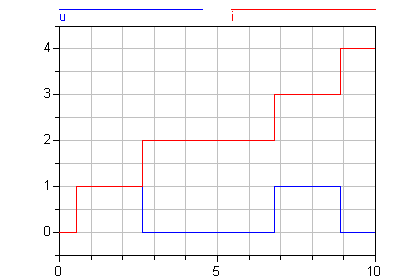
ModelicaReference.Operators.'change()'

Indicate discrete variable changing

Syntax

change(v)

Description

Is expanded into "(v<>pre(v))". The same restrictions as for the pre() operator apply.

Examples

model BothEdges
  Boolean u;
  Integer i;
equation
  u = Modelica.Math.sin(time) > 0.5;
  when change(u) then
    i = pre(i) + 1;
  end when;
end BothEdges;

Extends from ModelicaReference.Icons.Information (Icon for general information packages).

ModelicaReference.Operators.'connect()'

Connect objects

Examples

model Integrate
  Modelica.Blocks.Sources.Step step;
  Modelica.Blocks.Continuous.Integrator integrator;
equation
  connect(step.outPort, integrator.inPort);
end Integrate;

Example of array use:

connector InPort = input Real;

connector OutPort = output Real;

block MatrixGain
  input InPort u[size(A,1)];
  output OutPort y[size(A,2)]
  parameter Real A[:,:]=[1];
equation
  y=A*u;
end MatrixGain;

  sin sinSource[5];
  MatrixGain gain(A=5*identity(5));
  MatrixGain gain2(A=ones(5,2));
  OutPort x[2];
equation
  connect(sinSource.y, gain.u); // Legal
  connect(gain.y, gain2.u);     // Legal
  connect(gain2.y, x);          // Legal

Syntax

equation_clause :
  [ initial ] equation { equation ";" | annotation  ";" }

equation :
  ( simple_expression "=" expression
    | conditional_equation_e
    | for_clause_e
    | connect_clause
    | when_clause_e
    | IDENT function_call )
  comment

connect_clause :
  connect "(" component_reference "," component_reference ")"

Description

Connections between objects are introduced by the connect statement in the equation part of a class. The connect construct takes two references to connectors, each of which is either of the following forms:

c1.c2. ... .cn, where c1 is a connector of the class, n≥1 and ci+1 is a connector element of ci for i=1:(n-1).
m.c, where m is a non-connector element in the class and c is a connector element of m.

There may optionally be array subscripts on any of the components; the array subscripts shall be parameter expressions. If the connect construct references array of connectors, the array dimensions must match, and each corresponding pair of elements from the arrays is connected as a pair of scalar connectors.

The two main tasks are to:

Build connection sets from connect statements.
Generate equations for the complete model.

Definitions:

Connection sets
A connection set is a set of variables connected by means of connect clauses. A connection set shall contain either only flow variables or only non-flow variables.
Inside and outside connectors
In an element instance M, each connector element of M is called an outside connector with respect to M. All other connector elements that are hierarchically inside M, but not in one of the outside connectors of M, is called an inside connector with respect to M.
[Example: in connect(a,b.c) 'a' is an outside connector and 'b.c' is an inside connector, unless 'b' is a connector.]

Extends from ModelicaReference.Icons.Information (Icon for general information packages).

ModelicaReference.Operators.'Connections.branch()'

Defines required branch of spanning-tree

Syntax

Connections.branch(A.R,B.R);

Description

Defines a branch from the overdetermined type or record instance R in connector instance A to the corresponding overdetermined type or record instance R in connector instance B for a virtual connection graph. These branches are required to be part of the spanning-tree for the virtual connection graph (they do not directly generate equations, but should be combined with equations coupling A.R to B.R), whereas connect-statements are optional for the spanning-tree (and generate different equations depending on whether they are part of the spanning-tree or not).

Examples

This function can be used at all places where a connect(...) statement is allowed.

E.g., it is not allowed to use this function in a when-clause. This definition shall be used if in a model with connectors A and B the overdetermined records A.R and B.R are algebraically coupled in the model, e.g., due to B.R = f(A.R, <other unknowns>).

Extends from ModelicaReference.Icons.Information (Icon for general information packages).

ModelicaReference.Operators.'Connections.root()'

Defines a definite root node.

Syntax

Connections.root(A.R);

Description

The overdetermined type or record instance R in connector instance A is a (definite) root node in a virtual connection graph.

Examples

This definition shall be used if in a model with connector A the overdetermined record A.R is (consistently) assigned, e.g., from a parameter expressions.

Extends from ModelicaReference.Icons.Information (Icon for general information packages).

ModelicaReference.Operators.'Connections.potentialRoot()'

Defines a potential root node.

Syntax

Connections.potentialRoot(A.R);
Connections.potentialRoot(A.R, priority = p);

Description

The overdetermined type or record instance R in connector instance A is a potential root node in a virtual connection graph with priority p (with p ≥ 0). If no second argument is provided, the priority is zero. p shall be a parameter expression of type Integer. In a virtual connection subgraph without a Connections.root() definition, one of the potential roots with the lowest priority number is selected as root.

Examples

This definition may be used if in a model with connector A the overdetermined record A.R appears differentiated, der(A.R), together with the constraint equations of A.R, i.e., a non-redundant subset of A.R maybe used as states.

Extends from ModelicaReference.Icons.Information (Icon for general information packages).

ModelicaReference.Operators.'Connections.isRoot()'

Returns root status.

Syntax

b = Connections.isRoot(A.R);

Description

Returns true, if the overdetermined type or record instance R in connector instance A is selected as a root in the virtual connection graph.

Extends from ModelicaReference.Icons.Information (Icon for general information packages).

ModelicaReference.Operators.'Connections.rooted()'

Returns which node of a connection branch is closer to root.

Syntax

b = Connections.rooted(A.R);
b = rooted(A.R);  // deprecated

Description

If the operator Connections.rooted(A.R) is used, or the equivalent but deprecated operator rooted(A.R), then there must be exactly one statement Connections.branch(A.R,B.R) involving A.R (the argument of Connections.rooted must be the first argument of Connections.branch). In that case Connections.rooted(A.R) returns true, if A.R is closer to the root of the spanning tree than B.R; otherwise false is returned.

Examples

This operator can be used to avoid equation systems by providing analytic inverses, see Modelica.Mechanics.MultiBody.Parts.FixedRotation.

Extends from ModelicaReference.Icons.Information (Icon for general information packages).

ModelicaReference.Operators.'cos()'

Trigonometric cosine function

Syntax

cos(u)

Description

Returns the cosine of u, with -∞ < u < ∞ Argument u needs to be an Integer or Real expression.

The cosine function can also be accessed as Modelica.Math.cos.

Examples

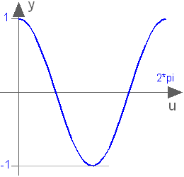
cos(3.14159265358979)
 = -1.0

Extends from ModelicaReference.Icons.Information (Icon for general information packages).

ModelicaReference.Operators.'cosh()'

Hyperbolic cosine function

Syntax

cosh(u)

Description

Returns the cosh of u, with -∞ < u < ∞. Argument u needs to be an Integer or Real expression.

The cosh function can also be accessed as Modelica.Math.cosh.

Examples

cosh(1)
  = 1.54308063481524

Extends from ModelicaReference.Icons.Information (Icon for general information packages).

ModelicaReference.Operators.'cross()'

Return cross product of two vectors

Syntax

cross(x, y)

Description

Returns the cross product of the 3-vectors x and y, i.e.

cross(x,y) = vector( [ x[2]*y[3]-x[3]*y[2];
                       x[3]*y[1]-x[1]*y[3];
                       x[1]*y[2]-x[2]*y[1] ] );

Extends from ModelicaReference.Icons.Information (Icon for general information packages).

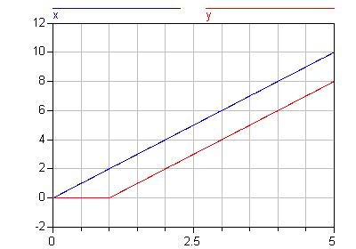
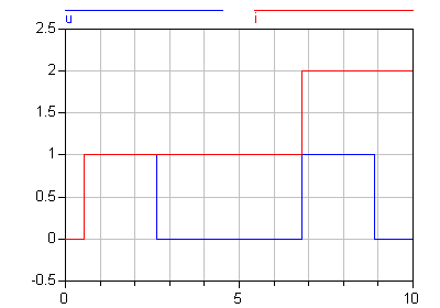
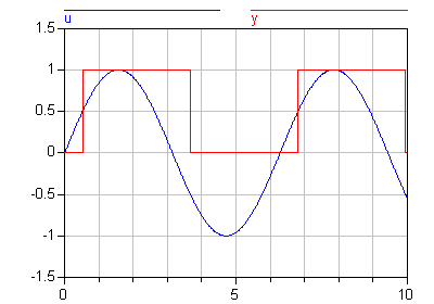
ModelicaReference.Operators.'delay()'

Delay expression

Syntax

delay(expr, delayTime, delayMax)
delay(expr, delayTime)

Description

Returns "expr(time - delayTime)" for time > time.start + delayTime and "expr(time.start)" for time ≤ time.start + delayTime. The arguments, i.e., expr, delayTime and delayMax, need to be subtypes of Real. delayMax needs to be additionally a parameter expression. The following relation shall hold: 0 ≤ delayTime ≤ delayMax, otherwise an error occurs. If delayMax is not supplied in the argument list, delayTime need to be a parameter expression.

[The delay operator allows a numerical sound implementation by interpolating in the (internal) integrator polynomials, as well as a more simple realization by interpolating linearly in a buffer containing past values of expression expr. Without further information, the complete time history of the delayed signals need to be stored, because the delay time may change during simulation. To avoid excessive storage requirements and to enhance efficiency, the maximum allowed delay time has to be given via delayMax, or delayTime must be a parameter expression (so that the constant delay is known before simulation starts). This gives an upper bound on the values of the delayed signals which have to be stored. For realtime simulation where fixed step size integrators are used, this information is sufficient to allocate the necessary storage for the internal buffer before the simulation starts. For variable step size integrators, the buffer size is dynamic during integration. In principal, a delay operator could break algebraic loops. For simplicity, this is not supported because the minimum delay time has to be give as additional argument to be fixed at compile time. Furthermore, the maximum step size of the integrator is limited by this minimum delay time in order to avoid extrapolation in the delay buffer.]

Examples

model Delay
  Real x;
  Real y;
equation
  der(x) = 2;
  y = delay(x, 1);
end Delay;

Extends from ModelicaReference.Icons.Information (Icon for general information packages).

ModelicaReference.Operators.'der()'

Time derivative of expression or
partial derivative of function

Syntax

der(expr) or
IDENT "=" der "(" name "," IDENT { "," IDENT } ")" comment

Description

The first form is the time derivative of expression expr. If the expression expr is a scalar it needs to be a subtype of Real. The expression and all its subexpressions must be differentiable. If expr is an array, the operator is applied to all elements of the array. For Real parameters and constants the result is a zero scalar or array of the same size as the variable.

The second form is the partial derivative of a function and may only be used as declarations of functions. The semantics is that a function [and only a function] can be specified in this form, defining that it is the partial derivative of the function to the right of the equal sign (looked up in the same way as a short class definition - the looked up name must be a function), and partially differentiated with respect to each IDENT in order (starting from the first one). The IDENT must be Real inputs to the function. The comment allows a user to comment the function (in the info-layer and as one-line description, and as icon).

Examples

  Real x, xdot1, xdot2;
equation
  xdot1 = der(x);
  xdot2 = der(x*sin(x));

The specific enthalpy can be computed from a Gibbs-function as follows:

function Gibbs
  input Real p,T;
  output Real g;
algorithm
  ...
end Gibbs;

function Gibbs_T=der(Gibbs, T);

function specificEnthalpy
  input Real p,T;
  output Real h;
algorithm
  h:=Gibbs(p,T)-T*Gibbs_T(p,T);
end specificEnthalpy;

Extends from ModelicaReference.Icons.Information (Icon for general information packages).

ModelicaReference.Operators.'diagonal()'

Returns a diagonal matrix

Syntax

diagonal(v)

Description

Returns a square matrix with the elements of vector v on the diagonal and all other elements zero.

Extends from ModelicaReference.Icons.Information (Icon for general information packages).

ModelicaReference.Operators.'div()'

Integer part of division of two Real numbers

Syntax

div(x, y)

Description

Returns the algebraic quotient x/y with any fractional part discarded (also known as truncation toward zero). [Note: this is defined for / in C99; in C89 the result for negative numbers is implementation-defined, so the standard function div() must be used.] Result and arguments shall have type Real or Integer. If either of the arguments is Real the result is Real otherwise Integer.

[Note, outside of a when clause state events are triggered when the return value changes discontinuously.]

Examples

div(13,6)
 = 2

Extends from ModelicaReference.Icons.Information (Icon for general information packages).

ModelicaReference.Operators.'edge()'

Indicate rising edge

Syntax

edge(b)

Description

Is expanded into "(b and not pre(b))" for Boolean variable b. The same restrictions as for the pre operator apply (e.g., not to be used in function classes).

Examples

model RisingEdge
  Boolean u;
  Integer i;
equation
  u = Modelica.Math.sin(time) > 0.5;
  when edge(u) then
    i = pre(i) + 1;
  end when;
end RisingEdge;

Extends from ModelicaReference.Icons.Information (Icon for general information packages).

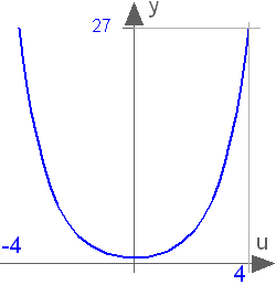
ModelicaReference.Operators.'exp()'

Exponential, base e.

Syntax

exp(u)

Description

Returns the base e exponential of u, with -∞ < u < ∞ Argument u needs to be an Integer or Real expression.

The exponential function can also be accessed as Modelica.Math.exp.

Examples

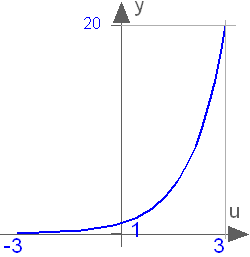
exp(1)
 = 2.71828182845905

Extends from ModelicaReference.Icons.Information (Icon for general information packages).

ModelicaReference.Operators.'fill()'

Return a Real, Integer, Boolean or String array with all elements equal

Syntax

fill(s, n1, n2, n3, ...)

Description

Returns the n1 x n2 x n3 x ... array with all elements equal to scalar or array expression s (ni >= 0). The returned array has the same type as s. Recursive definition:

fill(s,n1,n2,n3, ...) = fill(fill(s,n2,n3, ...), n1);
fill(s,n) = {s,s,..., s}

Examples

Real    mr[2,2] = fill(-1,2,2);  // = [-1,-1;-1,-1]
Boolean vb[3]   = fill(true,3);  // = {true, true, true}

Extends from ModelicaReference.Icons.Information (Icon for general information packages).

ModelicaReference.Operators.'floor()'

Round Real number towards minus infinity

Syntax

floor(x)

Description

Returns the largest integer not greater than x. Result and argument shall have type Real. [Note, outside of a when clause state events are triggered when the return value changes discontinuously.]

Examples

floor({-3.14, 3.14})
 = {-4.0, 3.0}

Extends from ModelicaReference.Icons.Information (Icon for general information packages).

ModelicaReference.Operators.'homotopy()'

During the initialization phase of a dynamic simulation problem, it often happens that large nonlinear systems of equations must be solved by means of an iterative solver. The convergence of such solvers critically depends on the choice of initial guesses for the unknown variables. The process can be made more robust by providing an alternative, simplified version of the model, such that convergence is possible even without accurate initial guess values, and then by continuously transforming the simplified model into the actual model. This transformation can be formulated using expressions of this kind:

lambda*actual + (1-lambda)*simplified

in the formulation of the system equations, and is usually called a homotopy transformation. If the simplified expression is chosen carefully, the solution of the problem changes continuously with lambda, so by taking small enough steps it is possible to eventually obtain the solution of the actual problem.

It is recommended to perform (conceptually) one homotopy iteration over the whole model, and not several homotopy iterations over the respective non-linear algebraic equation systems. The reason is that the following structure can be present:

w = f₁(x) // has homotopy operator
0 = f₂(der(x), x, z, w)

Here, a non-linear equation system f₂ is present. The homotopy operator is, however used on a variable that is an 'input' to the non-linear algebraic equation system, and modifies the characteristics of the non-linear algebraic equation system. The only useful way is to perform the homotopy iteration over f₁ and f₂ together.

The suggested approach is 'conceptual', because more efficient implementations are possible, e.g., by determining the smallest iteration loop, that contains the equations of the first BLT block in which a homotopy operator is present and all equations up to the last BLT block that describes a non-linear algebraic equation system.

A trivial implementation of the homotopy operator is obtained by defining the following function in the globalscope:

function homotopy
  input Real actual;
  input Real simplified;
  output Real y;
algorithm
  y := actual;
  annotation(Inline = true);
end homotopy;

Syntax

homotopy(actual=actual, simplified=simplified)

Description

The scalar expressions 'actual' and 'simplified' are subtypes of Real. A Modelica translator should map this operator into either of the two forms:

Returns 'actual' [a trivial implementation].
In order to solve algebraic systems of equations, the operator might during the solution process return a combination of the two arguments, ending at actual, e.g.,
```
actual*lambda + simplified*(1-lambda),
```
where lambda is a homotopy parameter going from 0 to 1.

The solution must fulfill the equations for homotopy returning 'actual'.

Examples

Example 1

In electrical systems it is often difficult to solve non-linear algebraic equations if switches are part of the algebraic loop. An idealized diode model might be implemented in the following way, by starting with a 'flat' diode characteristic and then move with the homotopy operator to the desired 'steep' characteristic:

model IdealDiode
  ...
  parameter Real Goff = 1e-5;
protected
  Real Goff_flat = max(0.01, Goff);
  Real Goff2;
equation
  off = s < 0;
  Goff2 = homotopy(actual=Goff, simplified=Goff_flat);
  u = s*(if off then 1     else Ron2) + Vknee;
  i = s*(if off then Goff2 else 1   ) + Goff2*Vknee;
  ...
end IdealDiode;

Example 2

In electrical systems it is often useful that all voltage sources start with zero voltage and all current sources with zero current, since steady state initialization with zero sources can be easily obtained. A typical voltage source would then be defined as:

model ConstantVoltageSource
  extends Modelica.Electrical.Analog.Interfaces.OnePort;
  parameter Modelica.SIunits.Voltage V;
equation
  v = homotopy(actual=V, simplified=0.0);
end ConstantVoltageSource;

Example 3

In fluid system modelling, the pressure/flowrate relationships are highly nonlinear due to the quadratic terms and due to the dependency on fluid properties. A simplified linear model, tuned on the nominal operating point, can be used to make the overall model less nonlinear and thus easier to solve without accurate start values. Named arguments are used here in order to further improve the readability.

model PressureLoss
  import SI = Modelica.SIunits;
  ...
  parameter SI.MassFlowRate m_flow_nominal "Nominal mass flow rate";
  parameter SI.Pressure     dp_nominal     "Nominal pressure drop";
  SI.Density                rho            "Upstream density";
  SI.DynamicViscosity       lambda         "Upstream viscosity";
equation
  ...
  m_flow = homotopy(actual     = turbulentFlow_dp(dp, rho, lambda),
                    simplified = dp/dp_nominal*m_flow_nominal);
  ...
end PressureLoss;

Example 4

Note that the homotopy operator shall not be used to combine unrelated expressions, since this can generate singular systems from combining two well-defined systems.

model DoNotUse
  Real x;
  parameter Real x0 = 0;
equation
  der(x) = 1-x;
initial equation
  0 = homotopy(der(x), x - x0);
end DoNotUse;

The initial equation is expanded into

0 = lambda*der(x) + (1-lambda)*(x-x0)

and you can solve the two equations to give

x = (lambda+(lambda-1)*x0)/(2*lambda - 1)

which has the correct value of x0 at lambda = 0 and of 1 at lambda = 1, but unfortunately has a singularity at lambda = 0.5.

Extends from ModelicaReference.Icons.Information (Icon for general information packages).

ModelicaReference.Operators.'identity()'

Returns the identity matrix of the desired size

Syntax

identity(n)

Description

Returns the n x n Integer identity matrix, with ones on the diagonal and zeros at the other places.

Extends from ModelicaReference.Icons.Information (Icon for general information packages).

ModelicaReference.Operators.'initial()'

True during initialization

Syntax

initial()

Description

Returns true during the initialization phase and false otherwise.

Examples

  Boolean off;
  Real x;
equation
  off = x < -2 or initial();

Extends from ModelicaReference.Icons.Information (Icon for general information packages).

ModelicaReference.Operators.'inStream()'

Returns the mixing value of a stream variable if it flows into the component where the inStream operator is used.

For an introduction into stream variables and an example for the inStream(..) operator, see stream.

Syntax

inStream(IDENT)

where IDENT must be a variable reference in a connector component declared with the stream prefix.

Description

In combination with the stream variables of a connector, the inStream() operator is designed to describe in a numerically reliable way the bi-directional transport of specific quantities carried by a flow of matter. inStream(v) is only allowed on stream variables v and is informally the value the stream variable has, assuming that the flow is from the connection point into the component. This value is computed from the stream connection equations of the flow variables and of the stream variables. For the following definition it is assumed that N inside connectors mj.c (j=1,2,...,N) and M outside connectors ck(k=1,2,...,M) belonging to the same connection set are connected together and a stream variable h_outflow is associated with a flow variable m_flow in connector c.

connector FluidPort
   ...
   flow   Real m_flow     "Flow of matter; m_flow > 0 if flow into component";
   stream Real h_outflow  "Specific variable in component if m_flow < 0"
end FluidPort;

model FluidSystem
   ...
   FluidComponent m1, m2, ..., mN;
   FluidPort      c1, c2, ..., cM;
equation
   connect(m1.c, m2.c);
   connect(m1.c, m3.c);
      ...
   connect(m1.c, mN.c);
   connect(m1.c, c1);
   connect(m1.c, c2);
      ...
   connect(m1.c, cM);
   ...
end FluidSystem;

With these prerequisites, the semantics of the expression

inStream(m_i.c.h_outflow)

is given implicitly by defining an additional variable h_mix_in_i, and by adding to the model the conservation equations for mass and energy corresponding to the infinitesimally small volume spanning the connection set. The connect equation for the flow variables has already been added to the system according to the connection semantics of flow variables:

// Standard connection equation for flow variables
0 = sum(m_j.c.m_flow for j in 1:N) + sum(-c_k.m_flow for k in 1:M);

Whenever the inStream() operator is applied to a stream variable of an inside connector, the balance equation of the transported property must be added under the assumption of flow going into the connector

// Implicit definition of the inStream() operator applied to inside connector i
0 = sum(m_j.c.m_flow*(if m_j.c.m_flow > 0 or j==i then h_mix_in_i else m_j.c.h_outflow) for j in 1:N) +
    sum(-c_k.m_flow* (if c_k.m_flow > 0 then h_mix_in_i else inStream(c_k.h_outflow) for k in 1:M);
inStream(m_i.c.h_outflow) = h_mix_in_i;

Note that the result of the inStream(m_i.c.h_outflow) operator is different for each port i, because the assumption of flow entering the port is different for each of them. Additional equations need to be generated for the stream variables of outside connectors.

// Additional connection equations for outside connectors
for q in 1:M loop
  0 = sum(m_j.c.m_flow*(if m_j.c.m_flow > 0 then h_mix_out_q else m_j.c.h_outflow) for j in 1:N) +
      sum(-c_k.m_flow* (if c_k.m_flow > 0 or k==q then h_mix_out_q else inStream(c_k.h_outflow)
          for k in 1:M);
  c_q.h_outflow = h_mix_out_q;
end for;

Neglecting zero flow conditions, the above implicit equations can be analytically solved for the inStream(..) operators. The details are given in Section 15.2 of the Modelica Language Specification version 3.2 Revision 1. The stream connection equations have singularities and/or multiple solutions if one or more of the flow variables become zero. When all the flows are zero, a singularity is always present, so it is necessary to approximate the solution in an open neighborhood of that point. [For example assume that m_j.c.m_flow = c_k.m_flow = 0, then all equations above are identically fulfilled and inStream(..) can have any value]. It is required that the inStream() operator is appropriately approximated in that case and the approximation must fulfill the following requirements:

inStream(m_i.c.h_outflow) and inStream(c_k.h_outflow) must be unique with respect to all values of the flow and stream variables in the connection set, and must have a continuous dependency on them.
Every solution of the implicit equation system above must fulfill the equation system identically [up to the usual numerical accuracy], provided the absolute value of every flow variable in the connection set is greater than a small value (|m₁.c.m_flow| > eps and |m₂.c.m_flow| > eps and ... and |c_M.m_flow| > eps).

In Section 15.2 a recommended implementation of the solution of the implicit equation system is given, that fulfills the above requirements.

Extends from ModelicaReference.Icons.Information (Icon for general information packages).

ModelicaReference.Operators.'Integer()'

Returns ordinal number of enumeration

Syntax

Integer(<expression of enumeration type>)

Description

Returns the ordinal number of the enumeration value E.enumvalue, to which the expression is evaluated, where Integer(E.e1) =1, Integer(E.en) =size(E), for an enumeration type E=enumeration(e1, ..., en).

Examples

type Size = enumeration(small, medium, large, xlarge);
Size tshirt = Size.large;
Integer tshirtValue = Integer(tshirt);  // = 3

Extends from ModelicaReference.Icons.Information (Icon for general information packages).

ModelicaReference.Operators.'integer()'

Round Real number towards minus infinity

Syntax

integer(x)

Description

Returns the largest integer not greater than x. The argument shall have type Real. The result has type Integer.

[Note, outside of a when clause state events are triggered when the return value changes discontinuously.]

Examples

integer({-3.14, 3.14})
 = {-4, 3}

Extends from ModelicaReference.Icons.Information (Icon for general information packages).

ModelicaReference.Operators.'linspace()'

Return Real vector with equally spaced elements

Syntax

linspace(x1, x2, n)

Description

Returns a Real vector with n equally spaced elements, such that

v[i] = x1 + (x2-x1)*(i-1)/(n-1) for 1 ≤ i ≤ n.

It is required that n ≥ 2. The arguments x1 and x2 shall be Real or Integer scalar expressions.

Examples

Real v[:] = linspace(1,7,4);  // = {1, 3, 5, 7}

Extends from ModelicaReference.Icons.Information (Icon for general information packages).

ModelicaReference.Operators.'log()'

Natural (base e) logarithm

Syntax

log(u)

Description

Returns the base e logarithm of u, with u > 0. Argument u needs to be an Integer or Real expression.

The natural logarithm can also be accessed as Modelica.Math.log.

Examples

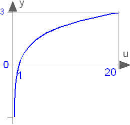
log(1)
 = 0

Extends from ModelicaReference.Icons.Information (Icon for general information packages).

ModelicaReference.Operators.'log10()'

Base 10 logarithm

Syntax

log10(u)

Description

Returns the base 10 logarithm of u, with u > 0. Argument u needs to be an Integer or Real expression.

The base 10 logarithm can also be accessed as Modelica.Math.log10.

Examples

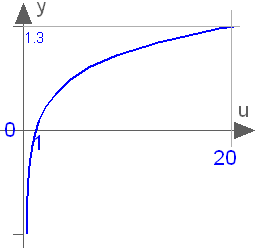
log10(1)
 = 0

Extends from ModelicaReference.Icons.Information (Icon for general information packages).

ModelicaReference.Operators.'matrix()'

Returns the first two dimensions of an array as matrix

Syntax

matrix(A)

Description

Returns promote(A,2), if A is a scalar or vector and otherwise returns the elements of the first two dimensions as a matrix. size(A,i) = 1 is required for 2 < i ≤ ndims(A).

Function promote(A,n) fills dimensions of size 1 from the right to array A up to dimension n, where "n > ndims(A)" is required. Let C = promote(A,n), with nA = ndims(A), then

ndims(C) = n,
size(C,j) = size(A,j) for 1 ≤ j ≤ nA,
size(C,j) = 1 for nA+1 ≤ j ≤ n,
C[i_1, ..., i_nA, 1, ..., 1] = A[i_1, ..., i_nA].

Extends from ModelicaReference.Icons.Information (Icon for general information packages).

ModelicaReference.Operators.'max()'

Returns the largest element

Syntax

max(A)
max(x,y)
max(e(i, ..., j) for i in u, ..., j in v)

Description

The first form returns the largest element of array expression A.

The second form returns the largest element of the scalars x and y.

The third form is a reduction expression and returns the largest value of the scalar expression e(i, ..., j) evaluated for all combinations of i in u, ..., j in v

Examples

max(i^2 for i in {3,7,6})  // = 49

Extends from ModelicaReference.Icons.Information (Icon for general information packages).

ModelicaReference.Operators.'min()'

Returns the smallest element

Syntax

min(A)
min(x,y)
min(e(i, ..., j) for i in u, ..., j in v)

Description

The first form returns the smallest element of array expression A.

The second form returns the smallest element of the scalars x and y.

The third form is a reduction expression and returns the smallest value of the scalar expression e(i, ..., j) evaluated for all combinations of i in u, ..., j in v

Examples

min(i^2 for i in {3,7,6})  // = 9

Extends from ModelicaReference.Icons.Information (Icon for general information packages).

ModelicaReference.Operators.'mod()'

Integer modulus of a division of two Real numbers

Syntax

mod(x, y)

Description

Returns the integer modulus of x/y, i.e., mod(x, y) = x - floor(x/y)*y. Result and arguments shall have type Real or Integer. If either of the arguments is Real the result is Real otherwise Integer. [Note, outside of a when clause state events are triggered when the return value changes discontinuously.]

Examples

mod(3,1.4)
 = 0.2
mod(-3,1.4)
 = 1.2
mod(3,-1.4)
 = -1.2

Extends from ModelicaReference.Icons.Information (Icon for general information packages).

ModelicaReference.Operators.'ndims()'

Return number of array dimensions

Syntax

ndims(A)

Description

Returns the number of dimensions k of array expression A, with k >= 0.

Examples

Real A[8,4,5];
Integer n = ndims(A);  // = 3

Extends from ModelicaReference.Icons.Information (Icon for general information packages).

ModelicaReference.Operators.'noEvent()'

Turn off event triggering

Syntax

noEvent(expr)

Description

Real elementary relations within expr are taken literally, i.e., no state or time event is triggered.

smooth vs. noEvent

The noEvent operator implies that real elementary expressions are taken literally instead of generating crossing functions. The smooth operator should be used instead of noEvent, in order to avoid events for efficiency reasons. A tool is free to not generate events for expressions inside smooth. However, smooth does not guarantee that no events will be generated, and thus it can be necessary to use noEvent inside smooth. [Note that smooth does not guarantee a smooth output if any of the occurring variables change discontinuously.]

[Example:

  Real x, y, z;
equation
  x = if time<1 then 2 else time-2;
  z = smooth(0, if time<0 then 0 else time);
  y = smooth(1, noEvent(if x<0 then 0 else sqrt(x)*x));
  // noEvent is necessary.

]

Examples

der(h)=if noEvent(h>0) then -c*sqrt(h) else 0;

Extends from ModelicaReference.Icons.Information (Icon for general information packages).

ModelicaReference.Operators.'ones()'

Returns an array with "1" elements

Syntax

ones(n1, n2, n3, ...)

Description

Return the n1 x n2 x n3 x ... Integer array with all elements equal to one (ni >=0 ).

Extends from ModelicaReference.Icons.Information (Icon for general information packages).

ModelicaReference.Operators.'outerProduct()'

Returns the outer product of two vectors

Syntax

outerProduct(v1,v2)

Description

Returns the outer product of vectors v1 and v2
(= matrix(v)*transpose( matrix(v) ) ).

Extends from ModelicaReference.Icons.Information (Icon for general information packages).

ModelicaReference.Operators.'pre()'

Refer to left limit

Syntax

pre(y)

Description

Returns the "left limit" y(t^pre) of variable y(t) at a time instant t. At an event instant, y(t^pre) is the value of y after the last event iteration at time instant t. The pre operator can be applied if the following three conditions are fulfilled simultaneously:

variable y is a subtype of a simple type
y is a discrete-time expression
the operator is not applied in a function class

The first value of pre(y) is determined in the initialization phase.

A new event is triggered if at least for one variable v "pre(v) <> v" after the active model equations are evaluated at an event instant. In this case the model is at once reevaluated. This evaluation sequence is called "event iteration". The integration is restarted, if for all v used in pre-operators the following condition holds: "pre(v) == v".

[If v and pre(v) are only used in when clauses, the translator might mask event iteration for variable v since v cannot change during event iteration. It is a "quality of implementation" to find the minimal loops for event iteration, i.e., not all parts of the model need to be reevaluated.

The language allows mixed algebraic systems of equations where the unknown variables are of type Real, Integer, Boolean, or an enumeration. These systems of equations can be solved by a global fix point iteration scheme, similarly to the event iteration, by fixing the Boolean, Integer, and/or enumeration unknowns during one iteration. Again, it is a quality of implementation to solve these systems more efficiently, e.g., by applying the fix point iteration scheme to a subset of the model equations.]

Note that pre(v) requires the argument to be a variable and a discrete-time expression, this formulation was chosen to allow using pre(v) both for discrete-time variables and for continuous-time variables inside when-clauses.

Examples

model Hysteresis
  Real u;
  Boolean y;
equation
  u = Modelica.Math.sin(time);
  y = u > 0.5 or pre(y) and u >= -0.5;
end Hysteresis;

Extends from ModelicaReference.Icons.Information (Icon for general information packages).

ModelicaReference.Operators.'product()'

Returns the scalar product

Syntax

product(A)
product(e(i, ..., j) for i in u, ..., j in v)

Description

The first form returns the scalar product of all the elements of array expression A:
A[1,...,1]*A[2,...,1]*....*A[end,...,1]*A[end,...,end]

The second form is a reduction expression and returns the product of the expression e(i, ..., j) evaluated for all combinations of i in u, ..., j in v:

e(u[1],...,v[1]) * e(u[2],...,v[1]) * ... *
e(u[end],...,v[1]) * ... * e(u[end],...,v[end])

The type of product(e(i, ..., j) for i in u, ..., j in v) is the same as the type of e(i,...j).

Examples

{product(j for j in 1:i) for i in 0:4} // = {1,1,2,6,24}

Extends from ModelicaReference.Icons.Information (Icon for general information packages).

ModelicaReference.Operators.'reinit()'

Reinitialize state variable

Syntax

reinit(x, expr)

Description

The operator reinitializes x with expr at an event instant. x is a Real variable (or an array of Real variables) that must be selected as a state (resp., states), that is reinit on x implies stateSelect = StateSelect.always on x. expr needs to be type-compatible with x. The reinit operator can for the same variable (resp. array of variables) only be applied (either as an individual variable or as part of an array of variables) in one equation (having reinit of the same variable in when and else-when of the same variable is allowed). The reinit operator can only be used in the body of a when-equation. It cannot be used in an algorithm section.

The reinit operator does not break the single assignment rule, because reinit(x,expr) in equations evaluates expr to a value (value), then at the end of the current event iteration step it assigns this value to x (this copying from values to reinitialized state(s) is done after all other evaluations of the model and before copying x to pre(x)).

[If a higher index system is present, that is constraints between state variables, some state variables need to be redefined to non-state variables. During simulation, non-state variables should be chosen in such a way that variables with an applied reinit operator are selected as states at least when the corresponding when-clauses become active. If this is not possible, an error occurs, since otherwise the reinit operator would be applied on a non-state variable.]

Examples

// Bouncing ball
   parameter Real e=0.5 "Coefficient of restitution"
   Real h, v;
   Boolean flying;
equation
   der(h) = v;
   der(v) = if flying then -g else 0;
   flying = not (h<=0 and v<=0);

   when h < 0 then
     reinit(v, -e*pre(v));
   end when;

Extends from ModelicaReference.Icons.Information (Icon for general information packages).

ModelicaReference.Operators.'rem()'

Integer remainder of the division of two Real numbers

Syntax

rem(x, y)

Description

Returns the integer remainder of x/y, such that div(x,y) * y + rem(x, y) = x. Result and arguments shall have type Real or Integer. If either of the arguments is Real the result is Real otherwise Integer. [Note, outside of a when clause state events are triggered when the return value changes discontinuously.]

Examples

rem(3,1.4)
 = 0.2
rem(-3,1.4)
 = -0.2
rem(3,-1.4)
 = 0.2

Extends from ModelicaReference.Icons.Information (Icon for general information packages).

ModelicaReference.Operators.'rooted()'

Deprecated operator, see Connections.rooted() instead.

Extends from ModelicaReference.Icons.Information (Icon for general information packages).

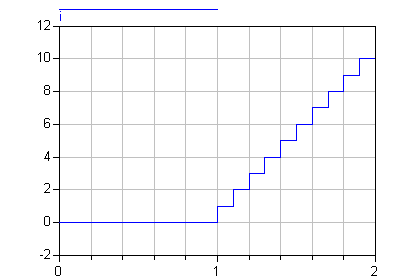
ModelicaReference.Operators.'sample()'

Trigger time events

Syntax

sample(start, interval)

Description

Returns true and triggers time events at time instants "start + i*interval" (i=0, 1, ...). During continuous integration the operator returns always false. The starting time "start" and the sample interval "interval" need to be parameter expressions and need to be a subtype of Real or Integer.

Examples

model Sampling
  Integer i;
equation
  when sample(1, 0.1) then
    i = pre(i) + 1;
  end when;
end Sampling;

Extends from ModelicaReference.Icons.Information (Icon for general information packages).

ModelicaReference.Operators.'scalar()'

Returns a one-element array as scalar

Syntax

scalar(A)

Description

Returns the single element of array A. size(A,i) = 1 is required for 1 ≤ i ≤ ndims(A).

Examples

Real A[1,1,1] = {{{3}}};
Real e = scalar(A);  // = 3

Extends from ModelicaReference.Icons.Information (Icon for general information packages).

ModelicaReference.Operators.'semiLinear()'

Returns "if x >= 0 then positiveSlope*x else negativeSlope*x" and handle x=0 in a meaningful way

Syntax

semiLinear(x, positiveSlope, negativeSlope)

Description

Returns "if x >= 0 then positiveSlope*x else negativeSlope*x". In some situations, equations with the semiLinear function become underdetermined if the first argument (x) becomes zero, i.e., there are an infinite number of solutions. It is recommended that the following rules are used to transform the equations during the translation phase in order to select one meaningful solution in such cases:

Rule 1: The equations

y = semiLinear(x, sa, s1);
y = semiLinear(x, s1, s2);
y = semiLinear(x, s2, s3);
   ...
y = semiLinear(x, sN, sb);

may be replaced by

s1 = if x >= 0 then sa else sb
s2 = s1;
s3 = s2;
   ...
sN = sN-1;
y = semiLinear(x, sa, sb);

Rule 2: The equations

x = 0;
y = 0;
y = semiLinear(x, sa, sb);

may be replaced by

x = 0
y = 0;
sa = sb;

[For symbolic transformations, the following property is useful (this follows from the definition):

semiLinear(m_flow, port_h, h);

is identical to

-semiLinear(-m_flow, h, port_h);

The semiLinear function is designed to handle reversing flow in fluid systems, such as

H_flow = semiLinear(m_flow, port.h, h);

i.e., the enthalpy flow rate H _flow is computed from the mass flow rate m_flow and the upstream specific enthalpy depending on the flow direction.]

Extends from ModelicaReference.Icons.Information (Icon for general information packages).

ModelicaReference.Operators.'sign()'

Sign function of a Real or Integer number

Syntax

sign(v)

Description

Is expanded into "noEvent(if v > 0 then 1 else if v < 0 then -1 else 0)". Argument v needs to be an Integer or Real expression.

Examples

sign({-3, 0, 3})
 = {-1, 0, 1}

Extends from ModelicaReference.Icons.Information (Icon for general information packages).

ModelicaReference.Operators.'sin()'

Trigonometric sine function

Syntax

sin(u)

Description

Returns the sine of u, with -∞ < u < ∞. Argument u needs to be an Integer or Real expression.

The sine function can also be accessed as Modelica.Math.sin.

Examples

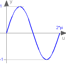
sin(3.14159265358979)
 = 0.0

Extends from ModelicaReference.Icons.Information (Icon for general information packages).

ModelicaReference.Operators.'sinh()'

Hyperbolic sine function

Syntax

sinh(u)

Description

Returns the sinh of u, with -∞ < u < ∞. Argument u needs to be an Integer or Real expression.

The sinh function can also be accessed as Modelica.Math.sinh.

Examples

sinh(1)
  = 1.1752011936438

Extends from ModelicaReference.Icons.Information (Icon for general information packages).

ModelicaReference.Operators.'size()'

Returns dimensions of an array

Syntax

   size(A,i)
   size(A)

Description

The first form returns the size of dimension i of array expression A where i shall be > 0 and ≤ ndims(A).

The second form returns a vector of length ndims(A) containing the dimension sizes of A.

Examples

Real A[8,4,5];
Integer n3   = size(A,3);  // = 5
Integer n[:] = size(A);    // = {8,4,5}

Extends from ModelicaReference.Icons.Information (Icon for general information packages).

ModelicaReference.Operators.'skew()'

Returns the skew matrix that is associated with a vector

Syntax

skew(x)

Description

Returns the 3 x 3 skew symmetric matrix associated with a 3-vector, i.e.,

cross(x,y) = skew(x)*y;
skew(x) = [ 0   , -x[3],  x[2];
            x[3],  0   , -x[1];
           -x[2],  x[1],  0   ];

Extends from ModelicaReference.Icons.Information (Icon for general information packages).

ModelicaReference.Operators.'smooth()'

Indicate smoothness of expression

Syntax

smooth(p, expr)

Description

If p>=0 smooth(p, expr) returns expr and states that expr is p times continuously differentiable, i.e.: expr is continuous in all real variables appearing in the expression and all partial derivatives with respect to all appearing real variables exist and are continuous up to order p.

The only allowed types for expr in smooth are: real expressions, arrays of allowed expressions, and records containing only components of allowed expressions.

smooth vs. noEvent

Examples

  Real x, y, z;
equation
  x = if time<1 then 2 else time-2;
  z = smooth(0, if time<0 then 0 else time);
  y = smooth(1, noEvent(if x<0 then 0 else sqrt(x)*x));
  // noEvent is necessary.

Extends from ModelicaReference.Icons.Information (Icon for general information packages).

ModelicaReference.Operators.'sqrt()'

Square root

Syntax

sqrt(v)

Description

Returns the square root of v if v>=0, otherwise an error occurs. Argument v needs to be an Integer or Real expression.

Examples

sqrt(9)
 = 3.0

Extends from ModelicaReference.Icons.Information (Icon for general information packages).

ModelicaReference.Operators.'String()'

Convert a scalar Real, Integer or Boolean expression to a String representation

Syntax

String(b_expr, minimumLength=0, leftJustified=true)
String(i_expr, minimumLength=0, leftJustified=true)
String(r_expr, significantDigits=6, minimumLength=0, leftJustified=true)
String(r_expr, format)
String(e_expr, minimumLength=0, leftJustified=true)

Description

The arguments have the following meaning (the default values of the optional arguments are shown in the left column):

Boolean b_expr

Boolean expression

Integer i_expr

Integer expression

Real r_expr

Real expression

type e_expr = enumeration(..)

Enumeration expression

Integer minimumLength = 0

Minimum length of the resulting string. If necessary,
the blank character is used to fill up unused space.

Boolean leftJustified = true

if true, the converted result is left justified;
if false, it is right justified in the string.

Integer significantDigits = 6

defines the number of significant digits in the result string
(e.g., "12.3456", "0.0123456", "12345600", "1.23456E-10")

String format

defines the string formatting according to ANSI-C without "%" and "*" character
(e.g., ".6g", "14.5e", "+6f"). In particular:
format = "[<flags>] [<width>] [.<precision>] <conversion>"
with

<flags>	zero, one or more of "-": left adjustment of the converted number "+": number will always be printed with a sign "0": padding to the field width with leading zeros
<width>	Minimum field width. The converted number will be printed in a field at least this wide and wider if necessary. If the converted number has fewer characters it will be padded on the left (or the right depending on <flags>) with blanks or 0 (depending on <flags>).
<precision>	The number of digits to be printed after the decimal point for e, E, or f conversions, or the number of significant digits for g or G conversions.
<conversion>	= "e": Exponential notation using a lower case e = "E": Exponential notation using an upper case E = "f": Fixed point notation = "g": Either "e" or "f" = "G": Same as "g", but with upper case E

Examples

String(2.0)   // = "2.0"
String(true)  // = "true"
String(123, minimumLength=6, leftJustified=false)  // = "   123"

Extends from ModelicaReference.Icons.Information (Icon for general information packages).

ModelicaReference.Operators.'sum()'

Returns the scalar sum

Syntax

sum(A)
sum(e(i, ..., j) for i in u, ..., j in v)

Description

The first form returns the scalar sum of all the elements of array expression A:
A[1,...,1]+A[2,...,1]+....+A[end,...,1]+A[end,...,end]

The second form is a reduction expression and returns the sum of the expression e(i, ..., j) evaluated for all combinations of i in u, ..., j in v:

e(u[1],...,v[1]) + e(u[2],...,v[1]) + ... +
e(u[end],...,v[1]) + ... + e(u[end],...,v[end])

The type of sum(e(i, ..., j) for i in u, ..., j in v) is the same as the type of e(i,...j).

Examples

sum(i for i in 1:10)  // Gives  1+2+...+10=55
   // Read it as: compute the sum of i for i in the range 1 to 10.

Extends from ModelicaReference.Icons.Information (Icon for general information packages).

ModelicaReference.Operators.'symmetric()'

Returns a symmetric matrix

Syntax

symmetric(A)

Description

Returns a matrix where the diagonal elements and the elements above the diagonal are identical to the corresponding elements of matrix A and where the elements below the diagonal are set equal to the elements above the diagonal of A, i.e.,

B := symmetric(A)
     -> B[i,j] := A[i,j], if i ≤ j,
        B[i,j] := A[j,i], if i > j.

Extends from ModelicaReference.Icons.Information (Icon for general information packages).

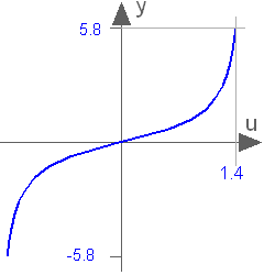
ModelicaReference.Operators.'tan()'

Trigonometric tangent function

Syntax

tan(u)

Description

Returns the tangent of u, with -∞ < u < ∞ (if u is a multiple of (2n-1)*pi/2, y = tan(u) is +/- infinity). Argument u needs to be an Integer or Real expression.

The tangent function can also be accessed as Modelica.Math.tan.

Examples

tan(3.14159265358979)
 = 0.0

Extends from ModelicaReference.Icons.Information (Icon for general information packages).

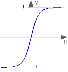
ModelicaReference.Operators.'tanh()'

Hyperbolic tangent function

Syntax

tanh(u)

Description

Returns the tanh of u, with -∞ < u < ∞. Argument u needs to be an Integer or Real expression.

The tanh function can also be accessed as Modelica.Math.tanh.

Examples

tanh(1)
  = 0.761594155955765

Extends from ModelicaReference.Icons.Information (Icon for general information packages).

ModelicaReference.Operators.'terminal()'

True after successful analysis

Syntax

terminal()

Description

Returns true at the end of a successful analysis.

Examples

  Boolean a, b;
equation
  a = change(b) or terminal();

Extends from ModelicaReference.Icons.Information (Icon for general information packages).

ModelicaReference.Operators.'terminate()'

Successfully terminate current analysis

Syntax

terminate(message)

Description

The terminate function successfully terminates the analysis which was carried out. The function has a string argument indicating the reason for the success. [The intention is to give more complex stopping criteria than a fixed point in time.]

Examples

model ThrowingBall
  Real x(start=0);
  Real y(start=1);
equation
  der(x)= ... ;
  der(y)= ... ;
algorithm
  when y < 0 then
    terminate("The ball touches the ground");
  end when;
end ThrowingBall;

Extends from ModelicaReference.Icons.Information (Icon for general information packages).

ModelicaReference.Operators.'transpose()'

Transpose of a matrix or permutation of the first two dimensions of an array

Syntax

transpose(A)

Description

Permutes the first two dimensions of array A. It is an error, if array A does not have at least 2 dimensions.

Extends from ModelicaReference.Icons.Information (Icon for general information packages).

ModelicaReference.Operators.'vector()'

Returns an array with one non-singleton dimension as vector

Syntax

vector(A)

Description

Returns a 1-vector, if A is a scalar and otherwise returns a vector containing all the elements of the array, provided there is at most one dimension size > 1.

Examples

Real A[1,2,1] = {{{3},{4}}};
Real v[2] = vector(A);  // = {3,4}

Extends from ModelicaReference.Icons.Information (Icon for general information packages).

ModelicaReference.Operators.'zeros()'

Returns a zero array.

Syntax

zeros(n1, n2, n3, ...)

Description

Returns the n1 x n2 x n3 x ... Integer array with all elements equal to zero (ni >= 0).

Extends from ModelicaReference.Icons.Information (Icon for general information packages).

Automatically generated Thu Dec 19 17:19:45 2019.